2.5. Weather Data Visualization with Ladybug (LB) Tools#
This tutorial demonstrates how to use the Ladybug plugin in Grasshopper to create a dashboard of climate analysis graphics from an EPW weather file. This process is fundamental for understanding the local climate and informing early-stage design decisions.
By the end of this tutorial, you will have created a set of visualizations in your Rhino viewport, which includes an hourly temperature plot, a monthly data chart, a psychrometric chart, a wind rose, and a sun path diagram for Van Nuys, California.
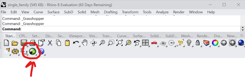
2.5.1. Open Grasshopper from Rhino by clicking the circled green icon.#
2.5.2. Place your first component.#
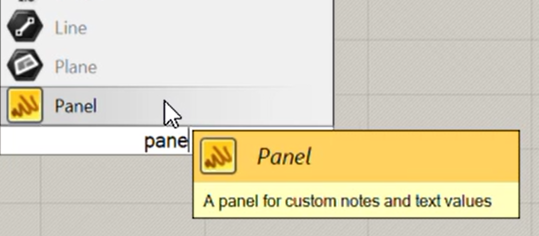
Double click on the Grasshopper canvas to search for components. Type in “Panel”. Click and drop the Panel onto the canvas.
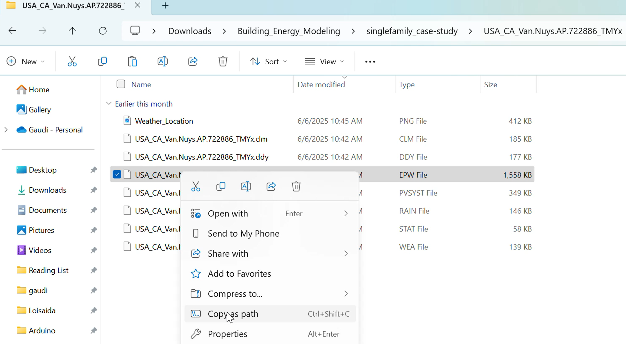
2.5.3. Locate your EnergyPlus Weather (epw) file in your file explorer and copy the file path as shown.#
Right click to open panel, then select “Copy as path”.
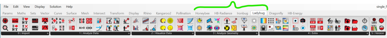
2.5.4. Plugin libraries and functions are located on the top bar.#
This is an alternative place to drag and drop components from.
2.5.5. Import EPW#
Double-click the canvas and type “LB Import EPW”. Select and place the ImportEPW component onto the canvas. Click and hold the right side of the panel where the small connection tab is located to create a connection. Drag and release onto the ImportEPW component connection tab to connect the components. This is the standard process of connecting components and will be referenced often throughout the modules.
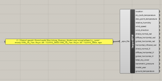
Notice the component name is located in the center of the “ImportEPW” component. To the left are inputs and to the right are outputs. Required inputs are denoted by a leading underscore (example: “_epw_file”). Connections determine the “flow” of data and operations. You can right click to inspect components. This can be useful for finding “runtime errors” and figuring out the next steps to solve them.
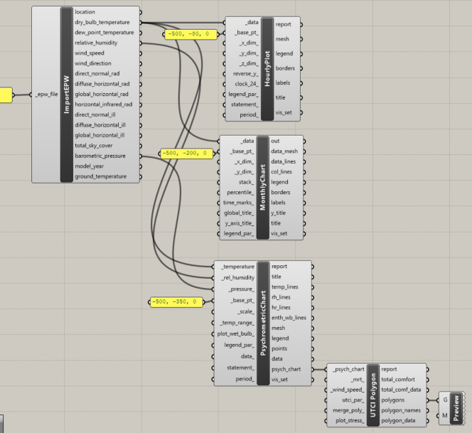
2.5.6. Create Temperature and Psychometric Charts.#
Practice double-clicking the canvas, searching for components (LB Hourly Plot, LB Monthly Chart, LB Psychronetric Chart, LB UTCI Polygon), selecting and placing them, and connecting them together to replicate the Grasshopper canvas shown below. Hover over the “_base_pt _” input and read the description to understand it’s purpose. The following modules will require you to replicate block diagrams in this way.
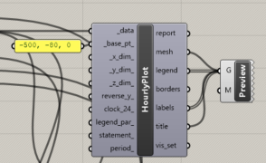
2.5.7. Hide lines in the hourly plot#
Right click the center of the LB Hourly Plot component and click the option to hide “Preview.” Then connect the indicated outputs to a “Custom Preview” component. Note how this removes the grid lines from the original plot. Custom Previews can be used to modify your plots.
2.5.8. Checking and understanding plots#
Once your components are properly connected, they will generate plots on your Rhino Canvas. It may be helpful to open a “Top” Rhino viewport and zoom out a bit to examine your plots. Double check that your three generated plots look like the plots below. If they are overlapping, revise your “_base_pt_input _”
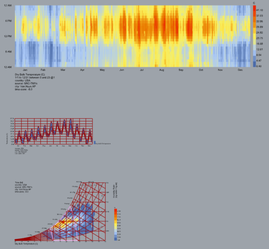
The plot on top (the hourly plot) is called an 8760 model. Each pixel represents one hour of the year. The legend on the right of the plot tells us that redder colors mean warmer temperatures and bluer colors mean colder temperatures. If we read the plot, we can see that it is generally colder at night, and the hottest temperatures are in the summer afternoons. This aligns with our real-life intuition.
Hover over the center of the other two plot components on your Grasshopper canvas to read about them.
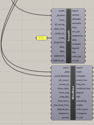
2.5.9. Create Wind Rose and Sun Path visualizations#
The _location input of “LB SunPath” component takes values from the _location output of your ImportEPW component. The _wind_direction input of “LB Wind Rose” takes values from the _wind_direction output of the ImportEPW component. The _data component takes values from the wind_speed output of ImportEPW. take better picture for this
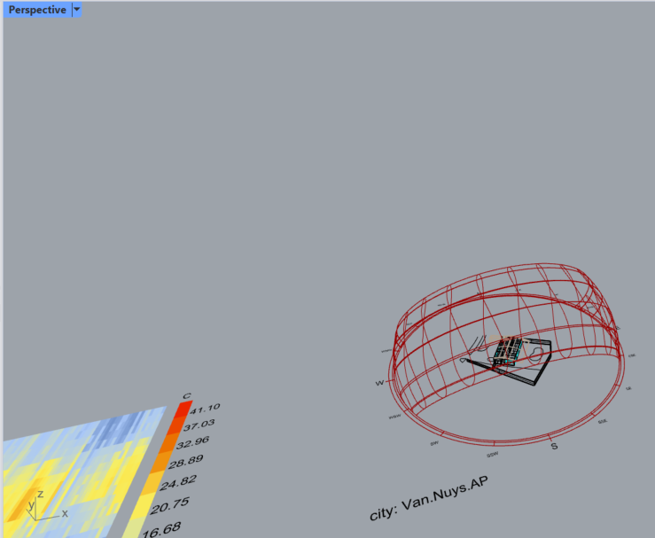
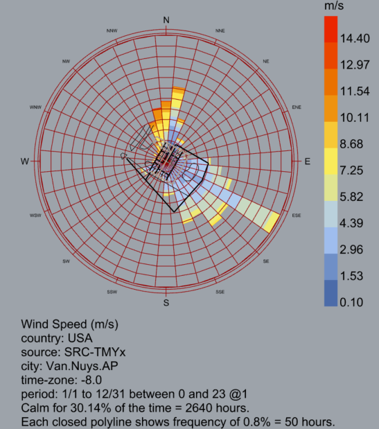
2.5.10. Check Wind Rose plot (perspective view)#
Investigate the wind rose in relation to your home. Manipulating a “Perspective” Rhino viewport may be useful here to explore the model. A wind rose visualizes the wind speed and direction at a specific location. This plot will be revisited in a later module.
2.5.11. Check Sun Path (perspective view)#
Investigate the sun path in relation to your home. Manipulating a “Perspective” Rhino viewport may be useful here to explore the model. A sun path diagram shows the sun’s path through the sky at a specific location. This plot will be revisited in a later module.