4.1. 8760 Models and Peak Loads#
4.1.1. Creating more 8760 visualizations#
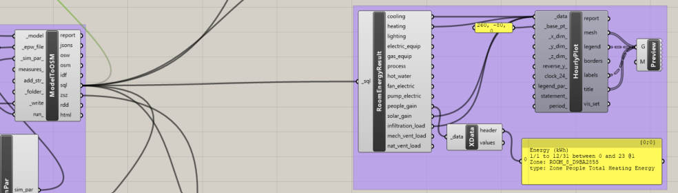
Recreate this block on your canvas. Explore connecting several RoomEnergyResult outputs to the _data input of Hourly Plot. Observe the generated plots. Use a LB Deconstruct Data (XData) component to see the header of the plots.
4.1.2. 8760 Plots#
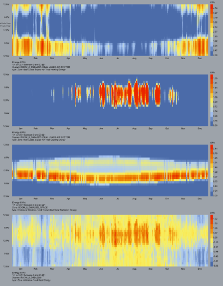
The image shows 8760 plots for heating, cooling, solar gain, and infiltration load. Do you notice any connections between the plots?
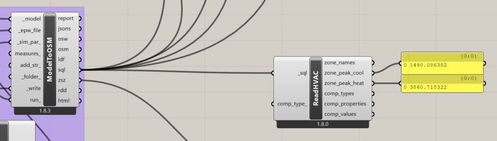
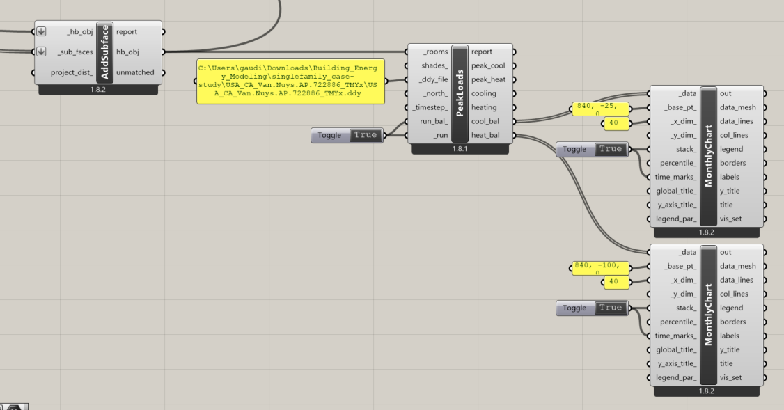
4.1.3. Calculating Peak Heating and Cooling Loads#
Follow along recreating the components (HB Read HVAC Sizing) and connections shown.
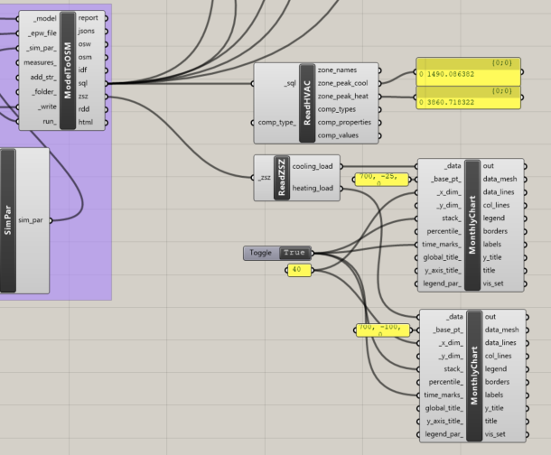
4.1.4. Visualizing Peak Heating and Cooling Loads#
Use a HB Read Zone Sizing (ReadZSZ) component.
4.1.5. Load Balances for Summer and Winter Design Days#
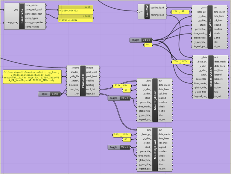
4.1.6. Double check Grasshopper blocks#
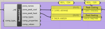
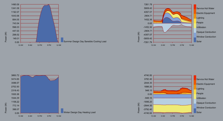
4.1.7. Peak Heating and Cooling Plots#
The left side plots show the cooling and heating load on the hottest and coldest days of the year. The right side plots double check that these plots have the right inputs and their interpretation.
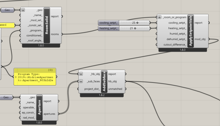
4.1.8. Set Heating and Cooling Setpoints#
The heating setpoint determines at what temperature the active heating system turns on. The cooling setpoint determines at what temperature the active cooling system turns on. This replicates the logic and behgavior of a thermostat. A heating setpoint of 21 C and a cooling setpoint of 25 C is reasonable for human comfort.
4.1.9. Vary Setpoints and Compare Calculated Peak Loads#
Note the peak heating and cooling loads for your chosen setpoints. Record them in a panel. Then change your setpoints and compare the calculated peak loads. How do they change? Does this align with your expectations?