3.1. Loads and EUI Simulation#
3.1.1. Model to OSM component#
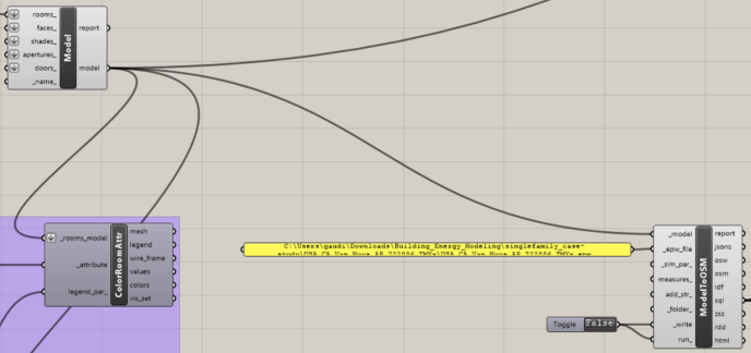
Recreate the components (HB Model to OSM, Boolean Toggle, Panel) and connections as shown below. Leave yourself some space in the canvas for future components. Note the toggle component is left as false and connected to both write and run. Leaving this toggle as false will prevent early simulation runs which take a few seconds to load.
3.1.2. Simulation Parameters components#
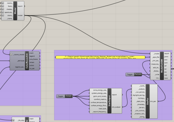
Continue recreating the components (HB Simulation Output, HB Simulation Parameter, Boolean Toggle) and connections shown in the images step-by-step.
3.1.3. Room Energy Result#
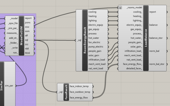
Note the several outputs of the “HB Model to OSM” component. We will use the sql output the most in future modules. Think of this as the main simulation data. There is a ton of data contained here. We will route this vast data to other components (HB Read Face Result, HB Read Room Energy Result) to preform operations on and visualize specific parts of the data.
3.1.4. Monthly Load Balance Visualization#
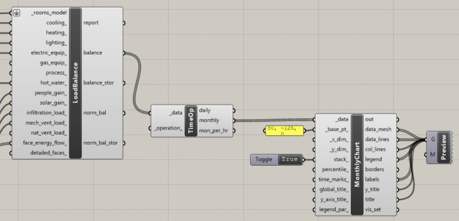
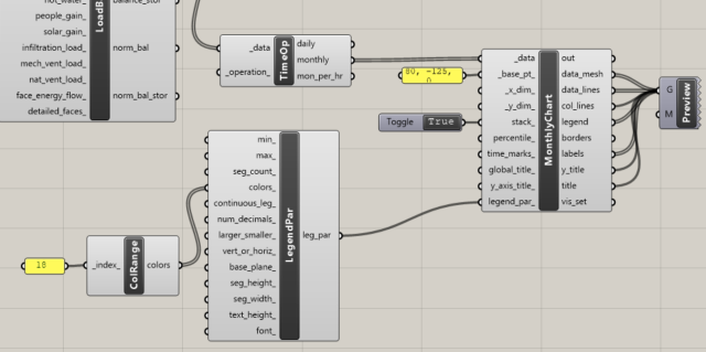
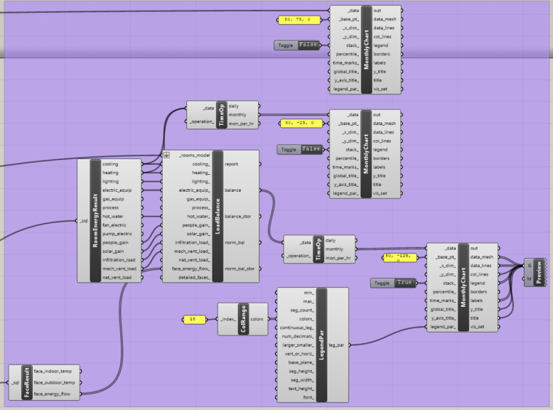
Connect the model output of “HB Model” to _rooms_model input of “HB Thermal Load Balance.” Create a “LB Time Interval Operation” component such that it takes in the load balance and performs a monthly time interval operation on the data collection. Input that into the “LB Monthly Chart” to visualize the monthly load balance.
3.1.5. Legend Parameters#
Insert a “LB Legend Parameter” component whose input colors are dictated by “LB Color Range” which creates gradient visualizations.
3.1.6. Load Balance Plot#
This is the load balance plot which should be generated in your Rhino viewport. To see this plot, it may be helpful to open a new “Top” Viewport, maximize it, and zoom out a bit.
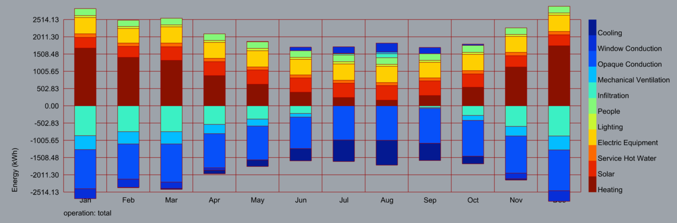
This plot shows the heat gains and losses colored by source for each month. Notice that the heat gains cancel out the heat losses. This means by the end of each month we finish at the same temperature we started. We see that more energy is used for “Heating” than “Cooling”. This represents the required active heating and cooling that would be preformed by an HVAC system. Notice the “Infiltration” source in teal. Read more about that here: https://en.wikipedia.org/wiki/Infiltration_(HVAC)
3.1.7. Heating and Cooling Loads Visualization#
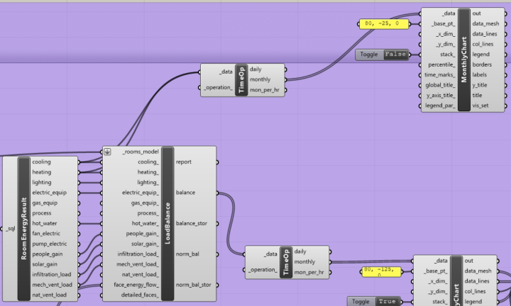
The “TimeOp” component takes both heating and cooling data from EnergyResult as inputs to _data.
3.1.8. Dry Bulb Temp Visualization#
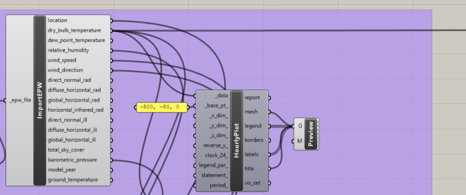
Create a new monthly chart with an appropriate base_pt _. Connect the dry_bulb_temperature output of your ImportEPW component to the _data input of your new monthly chart. This creates a monthly chart that shows the temperature readings using a standard thermometer that is not affected by the moisture in the air, aka a dry bulb. Knowing dry bulb temperature is important in building design when considering thermal comfort, implementing HVAC systems, and assessing heat stress. Another view of this configuration is shown in the next image.
3.1.9. Double-check Canvas#
This is what your plot generation logic should look like.
3.1.10. Monthly Heating and Cooling Loads Plot with Temperature#
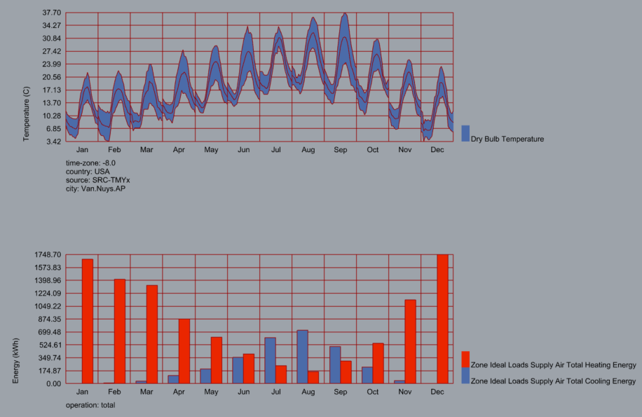
This is what your second and third generated plots should look like. The top shows average daily temperatures by month. The bottom shows heating and cooling loads for each month. We have higher heating loads in the winter and higher cooling loads in the summer.
Consider the results. Does this align with what you would expect?
3.1.11. Finding Construction and Program Sets#
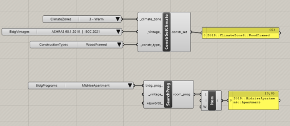
Explore the drop down menus to find an appropriate construction set. For our case study, we are in Van Nuys, California which is in Climate Zone 3 (add reference). We can choose a newer vintage to start, assuming the home was built recently.
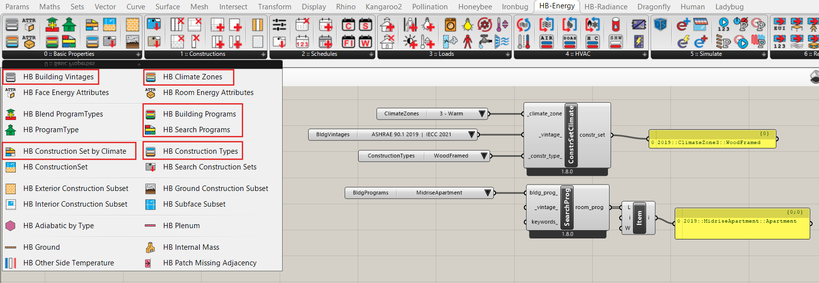
Here is another reference image including the HB Panel where you can drag and drop many of these components from.
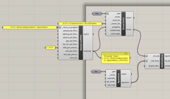
3.1.12. Connect Sets to Room Definition#
We can copy and paste the program and construction set values into a panel for accessibility. Then we can connect these panels to our main workflows. This leaves, the drop down menus free to explore without triggering a new simulation accidentally.
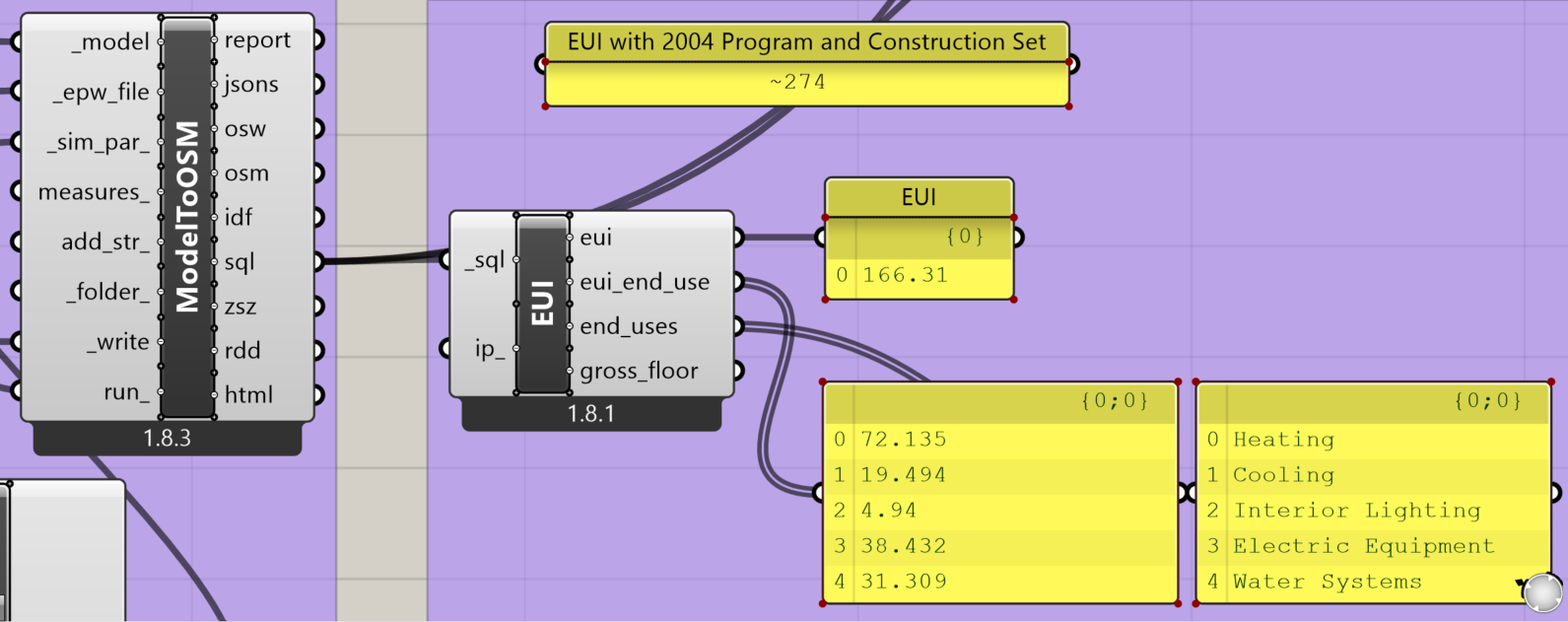
3.1.13. Compare EUI for Different Vintages#
When evaluating building energy efficiencies, the term EUI will appear across many times. EUI, in most cases, stands for Energy Use Intensity, calculated by dividing the total annual energy consumption (kWh) by the total gross floor area (m2). However, this could easily be confused with End-Use Intensity, which breaks down that total annual energy consumption into specific uses (i.e. heating, cooling, lighting, appliances), also in SI units of kWh/m2.
Using “HB End Use Intensity” component, try recording your simulation EUI with your building vintage of choice. When you change the vintage, ensure these construction sets are reflected in the panels attatched to your main workflow. Compare the EUI side by side. Do your results align with your expectations?
Hover over the ip input to view what units of measure are available. Without a Boolean Toggle, it defaults to False which produces results in kWh/m2. To change to Imperial System Units (IP), set Toggle to True in order to get the EUI in terms of kBtu/ft2.